Hi all, it’s been some time since I last wrote anything on this blog. This time around I’d like to share some experience that I’ve had with my recent hobby project: high quality time domain audio compression using DPCM (Differential Pulse-Code Modulation).
Be warned: this is quite a lengthy post.
tl;dr version: A Dynamic Differential Pulse-Code Modulation (DDPCM) method is presented. The method generally gives CD quality audio with about 8 bits / sample (compression ratio 2:1), and close-to CD quality with 4 bits / sample (compression ratio 4:1), using a super-simple branchless decoder. Sound examples here, and a C++ reference implementation here.
Background
I started looking into DPCM recently mainly because of discussions going on in the W3C Web Audio working group dealing with reducing the memory footprint of audio samples in a real-time audio engine (e.g. for game sound effects and music instruments).
I came to think about how 3D hardware supports various texture compression techniques in order to save GPU memory, and figured that a similar strategy could be successful for an audio engine too.
Goals
I roughly had the following goals for the compression algorithm:
- The data should be seekable (almost random access) in order to support variable playback rates, interpolation, looping, reverse playback etc.
- The decompression routine should be very light-weight, with fairly constant CPU-load (e.g. don’t introduce occasional CPU load spikes when decoding large buffers).
- The sound quality should be indistinguishable from CD quality.
- The data size should be roughly half of CD quality data. In other words, I aimed for 8 bits per sample whereas a CD uses 16 bits per sample.
- The compression routine should be light-weight too – enough so to enable on-demand compression, e.g. when loading assets.
Since DPCM with non-linear 8-bit quantization basically fulfills all those goals, that became my starting point.
Restart points
One thing worth noting is that in order to support seeking, you can’t just store a long series of delta values. You need restart points at regular intervals too so that you don’t have to accumulate N delta values to reach sample number N. For instance, with restart points every 16 samples, you have to accumulate at most 15 delta values to decode any single sample.
Quantization
The trickiest part of a DPCM coder/decoder is the quantization function, which is also the key to good sound quality. In other words: How do you map a delta value in the range [-65535, +65535] to an 8-bit code (and vice versa)?
There are several different DPCM formats/implementations. The key difference between the different formats is the quantization function, which is often described as a fixed look-up-table. See for instance:
The RoQ quantization function is quite simple and analytical. In principle, delta = code², so codes 0, 1, 2, 3, 4, …, 127 map to delta values 0, 1, 4, 9, 16, …, 16129. Reasonable and logical.
However, looking at the Interplay solution, we see a completely different picture: The look-up-table does not appear to have analytical origins. It’s not even continuous, and even worse: it contains duplicates! My gut feeling was that this table must have been generated statistically somehow.
This got me thinking: What’s the optimal quantization function? And how can I find that optimal function?
Step 1: Statistical analysis
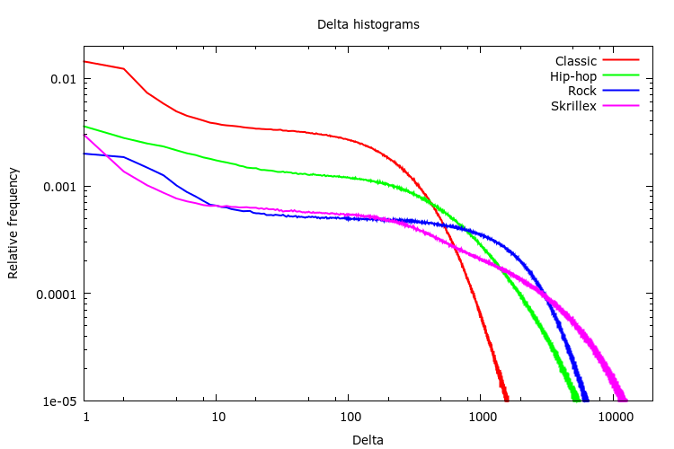
Since we want to quantize delta values, let’s start by looking at how common different delta values are. A histogram does the trick. I created histograms of sample deltas for a few different musical pieces, just to see if there are any similarities (the more similar the histograms are, the more likely it is that we can find a universal quantization function).
As you can see, small deltas are typically more common than large deltas. This is to be expected since natural sound and music typically has more energy in low frequencies (producing small deltas) than in high frequencies (producing large deltas).
On the other hand, the histograms for different pieces of music look quite different from each other. This may indicate that it will be difficult to find one universal, fixed quantization function that works well for all kinds of sound (more on that later).
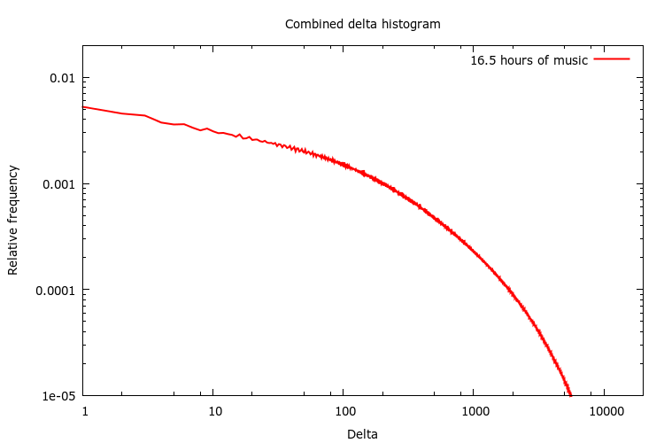
Figuring that more is merrier, I dug out a set of CD records that I had at home. I tried to pick records with varying style: rock, pop, classical, hip-hop, etc, ranging from Frank Sinatra and Barbara Streisand to Metallica and Prodigy. To top it off, I added the audio track of Elephants Dream (it’s a nice mix of sound effects, speech and music). All in all, I collected 9.8 GB of lossless CD quality audio (that’s about 16.5 hours).
Here’s what the combined histogram looks like:
Step 2: Creating an optimal quantization table
Now that we have a histogram, how can we turn it into a quantization table? This basically boils down to the definition of “optimal”.
What if the “optimal quantization function” would mean the function that would minimize the RMS error of the quantized data? Sounds about right!
Without doing too much thinking, I tried a greedy algorithm that worked really well. It goes like this:
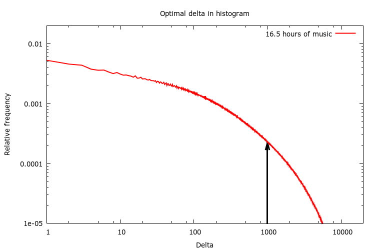
Imagine that we wanted to find a single delta value that best represents the entire histogram. Then just try all possible delta values (0 to 65535) and pick the one that would give the smallest RMS error for the given histogram. In my case, it landed pretty close to delta = 1000.
Given that single delta value, we could encode all deltas with a single bit of information (0 -> +delta, 1 -> -delta), but of course that would introduce quite a big quantization error on average.
With 8 bits for each quantized code we want 128 unique delta values (and then we add another 128 values that are equal to the first 128 values but with a negative sign, for a total of 256 unique delta values).
To find these extra levels, we split the histogram into two where we found the optimal delta value, and repeat the process for each half of the histogram. And then we recursively continue until we have the number of levels that we want.
By limiting the recursion depth to 7 we get 127 (2^7 – 1) splits. But we wanted 128 delta values… The solution is to do a final pass over all the 128 intervals defined by the 127 splits.
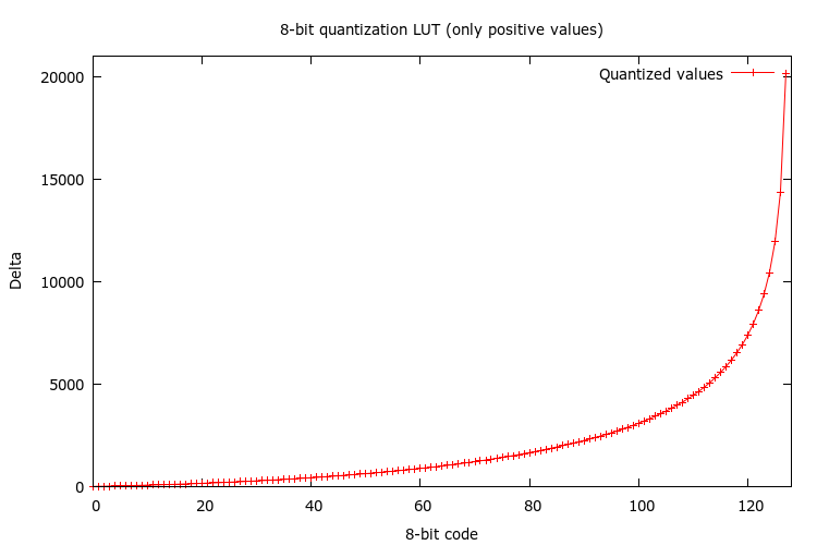
Using this method, I got the following quantization table (the 128 positive values):
1, 5, 10, 15, 21, 28, 34, 41,
48, 55, 63, 71, 79, 88, 96, 105,
114, 123, 133, 143, 153, 164, 175, 186,
197, 208, 220, 233, 246, 259, 272, 286,
300, 315, 330, 345, 360, 376, 393, 410,
427, 445, 463, 482, 501, 520, 540, 561,
582, 603, 626, 649, 672, 695, 720, 745,
770, 796, 823, 850, 879, 908, 937, 967,
999, 1032, 1067, 1102, 1138, 1175, 1212, 1251,
1290, 1331, 1373, 1416, 1461, 1506, 1553, 1602,
1651, 1702, 1755, 1810, 1866, 1923, 1983, 2044,
2107, 2173, 2241, 2311, 2384, 2459, 2537, 2618,
2703, 2793, 2887, 2984, 3086, 3192, 3304, 3422,
3545, 3675, 3812, 3956, 4109, 4272, 4446, 4632,
4833, 5054, 5294, 5555, 5842, 6159, 6514, 6913,
7376, 7923, 8577, 9384, 10440, 11931, 14354, 20162
Step 3: Introducing Dynamic DPCM (DDPCM)
The fixed quantization function developed above seems to be optimal on average. Still, sounds are usually quite different, and even a single piece of sound (e.g. a five seconds section of a piece of music) has a lot of dynamics (e.g. virtually silent vs snare drum vs flute vs vocals). What if we could use different quantization functions for different parts of a sound, in order to be locally optimal?
Idea 1: The encoded data is already divided into short blocks with restart markers. We could add a few extra bits of information to each block that tells the decoder which quantization table to use.
Idea 2: Let’s create a few different histograms based on the local average delta. I.e. for each section of N samples in the training set, find the average delta value, and based on that average delta value, select which histogram to update. Then, turn each histogram into a separate quantization table according to the method described above.
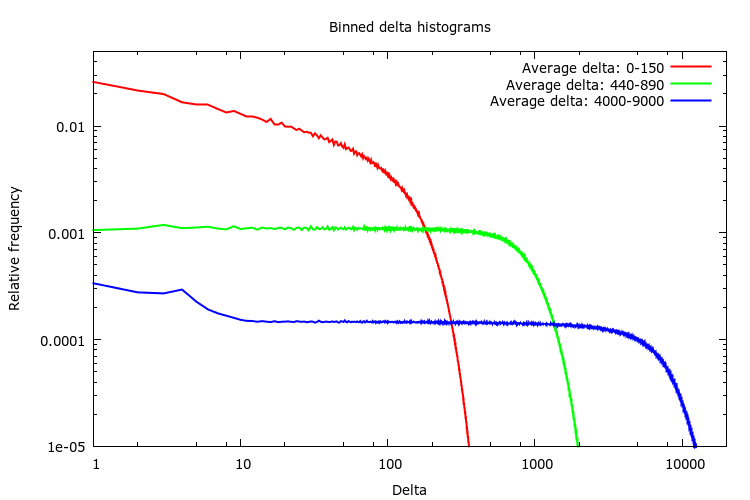
Here are a few histograms of the training set, each representing all 16-sample blocks in the training set with an average delta within a certain range:
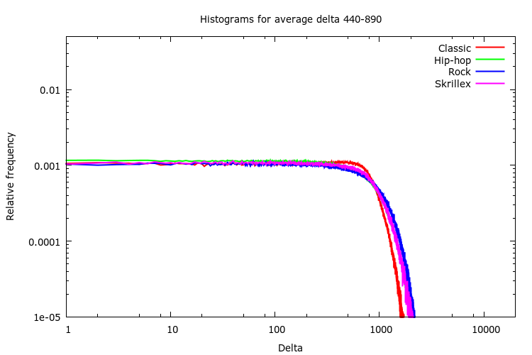
What if we look at a certain average delta interval for different pieces of music?
As you can see, they are actually quite similar. This is good news! That means that if we derive a quantization table from such a histogram, it’s quite likely that it will be a good fit regardless of what piece of sound or music we try to encode.
Mostly based on intuition and tweaking, I ended up using eight different histograms, resulting in eight quantization tables.
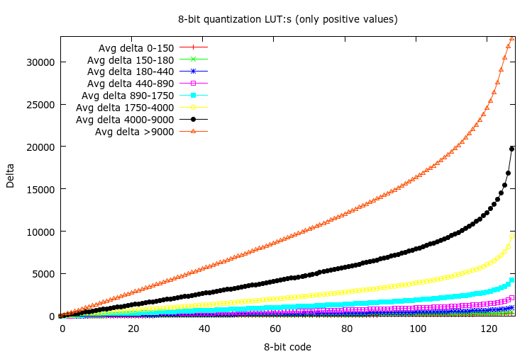
Selecting the average delta intervals was a bit tricky. I noticed that all the quantization tables had a predominant linear part, and I ended up manually adjusting the average delta intervals so that I got quantization tables with the slopes 1, 2, 4, 8, 16, 32, 64 and 128 (roughly).
Given that the tables are so similar to each other (except for the scaling factor), an interesting exercise would be to use a single quantization table in combination with a per-block bit-shift operation in the decoder instead of a per-block quantization table.
At this point, it’s pretty much impossible to hear the difference between the original 16-bit PCM sound and the 8-bit DDPCM sound. And the decoder is dead simple!
Step 4: The 4-bit version
After having tuned the 8-bit DDPCM scheme for a while, I thought to myself: “What if we just use 4 bits per delta?”. That would mean a compression ratio of 4:1, so it’s certainly attractive. But what about the sound quality?
With a few quick hacks, and some tweaking, I arrived at a solution that uses 64 quantization tables (as compared to the 8 tables in the 8-bit case). Each table is of course smaller (only 16 values / table), amounting to 2 KB of constant data in the decoder (using 16-bit signed integers for the table elements). Also, in order to lessen the relative overhead of the block restart data, the block length was extended from 16 to 32 samples per block.
Having more quantization tables at hand typically reduces the quantization error, since it’s possible to find a better fit for each individual block.
The result was surprisingly good, at least to me. But when comparing it to 4-bit MS ADPCM (I used sox -e ms-adpcm for creating the ADPCM WAVE file), my 4-bit DDPCM would give slightly worse quality, at least for “clean” sounds (e.g. a solo piano).
Step 5: A better predictor
In classic DPCM each sample is predicted to be the same as the previous sample, and what needs to be encoded is the difference from that prediction (i.e. the delta to the previous sample). By taking more samples into account it’s possible to do better predictions and thus reduce the power of the signal that has to be encoded.
Since I was pretty sure that the main reason for MS ADPCM’s better quality in some situations was that it has a more advanced predictor, I went ahead and did a quick test with a higher order predictor.
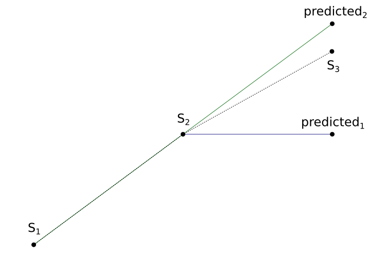
The figure below shows the two different predictors. S1 and S2 are known sample points, and S3 is the sample point that we need to encode next. Using the standard “delta” method in DPCM, we estimate S3 as predicted1. By using linear extrapolation instead, we arrive at predicted2.
Using the linear extrapolation predictor usually makes a huge difference for clean sounds. On the other hand it can actually make the situation worse for non-smooth data (e.g. noise, sharp transients and high frequencies). The solution: select the best predictor on a per-block basis. Since we only have two different predictors (“previous sample” and “linear extrapolation”) we only have to add one extra bit of information in the block.
The result? As far as I can tell 4-bit DDPCM outperforms 4-bit MS ADPCM in pretty much every aspect (RMS error, dynamic range etc), and it’s usually “good enough” for casual listening or sound effects.
Examples and source code
To check a couple of sound examples, go to the SAC audio demos page.
I have written a small reference implementation in C++ that does encoding and decoding. Feel free to try it out: https://gitlab.com/mbitsnbites/libsac
Dear sir,
I have some wave files.
May you help me to encode these files and decode them using 4-bit DDPCM?
I want to listen the quality.
thanks.
I think that the easiest way is to try the experimental SAC conversion tool (command line tool). You can find links to the source code and pre-compiled executables for 64-bit Windows and Linux at sac.bitsnbites.eu.
Note: The tool only supports 16-bit PCM WAVE files. Run the tool from a command line to get instructions.
Dear Sir,
May you provide me the training tool to create quantization table?
The table in the code is not good for low sampling rate.
Thanks.
Jason, I’d love to, but the “tool” is not really in a useful state (if it was I would have open sourced it). You will most likely have greater success implementing your own tool based on the information in this blog.
Have you tested your method against 8-bit data? I’ve been experimenting with 4:1 schemes for 8-bit PCM and am finding typical ADPCM schemes deficient.
No, I haven’t tried it with 8-bit data. The DDPCM method is optimized for reproducing a high dynamic range, which typically requires about 16 bits or more in the PCM representation.
4:1 for 8-bit PCM seems like a good challenge (i.e. 2 bits per sample), but I doubt that any form of DPCM would be sufficient. I’d start looking at more advanced data transformations, such as frequency domain representations, and / or hybrid methods (there’s some interesting work in Opus).
My target platform is way too slow for those, but thanks for the suggestions. I already have a few alternate schemes working, but will keep experimenting with dpcm.
in MS ADPCM you can specify the blocksize per file. (A typical block is 500 samples.)
This makes it quite hard to compare only on quality since this is basicly compression tradeof.
EG ms-adpcm filesizes:
blocksize 5 = compress to 100 %
blocksize 50 = compress to 31%
blocksize 500 = compress to 25.6 %
Did you look at encoding left + right stereo signals as mid+side?
The psychoacoustic basis for this, is that you could allocate relatively fewer bits to the side output, as the ear should be relatively less fussy about stereo separation than the main signal. FM Stereo radio has used this principle for 40+ years.
That’s really quite an astounding result, especially the 4-bit version, I really wasn’t expecting that..
There does however seem to be a bug somewhere.. Testing it on sounds that fade to digital silence results in weird noise once into true digital silence.. I will have a dig through the code tomorrow, because I’m curious..
8bit has this effect, though much quieter (almost inaudible) than the 4bit version..
In particular the EBU SQAM 35 Glockenspiel test file is guilty of this..
EBU SQAM test CD files are available here:
https://tech.ebu.ch/publications/sqamcd
Amazing work, can’t believe it took me so long to come across it..
Do you think it would make much difference having a separate set of maps for the predicted vs non predicted deltas ?
I think that there may be bugs in the code. I recall getting some “pop”:s during near silence.
Since I considered this a proof-of-concept I didn’t work more on the codec quality etc (it should not be too hard to re-implement it from scratch based on the look-up-tables that I created), but nevertheless I’m quite happy with the result.
In theory it should be better to use different maps for the different predictors. IIRC I did a quick hack to test it, but it resulted in worse results. That could very well be a mistake / bug on my part, though, so it’s definitely something worth looking into.
Another interesting area of research would be to do the same exercise with different sample rates (the tables that I got are tuned for 44100 samples/s). E.g. 11050 samples/s could be an interesting low bandwidth target (but probably harder, since there’s usually more entropy in lower sample rate audio).